Statistics

AP Statistics FRQ Practice

Nine original free-response questions, one for each AP Statistics unit — each with a model solution, AP-style scoring notes and a printable PDF — plus video walkthroughs of released exam questions.

9practice FRQs
1per AP unit
6exam walkthroughs
🆓PDF + answer key
🎬
Watch
Bilingual video lessons
English & Filipino
📄
Worksheet
Aligned practice problems
for every lesson
⬇
Download
Free PDF — print it or
solve it digitally

Watching in: English — toggle to switch video links

Each question below is written in the style of an AP Statistics free-response question and takes about 13 minutes. Try it on paper first, then open the model solution and score yourself the way AP readers do: E (essentially correct), P (partially correct) or I (incorrect) for each part. Every question has a printable PDF with the answer key.

These are original Numberbender practice questions with hypothetical data — not official College Board questions. For released exam questions and their scoring guidelines, see AP Central.

Unit 1

Minutes Spent on a Pre-Class Video

Exploring One-Variable Data

A math teacher who uses a flipped classroom recorded how many minutes each of 15 students spent watching the pre-class video for one lesson. The times, in minutes, are listed below.

Minutes
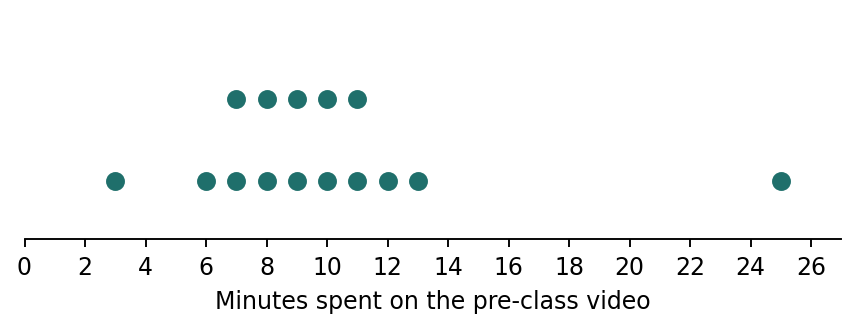
3, 6, 7, 7, 8, 8, 9, 9, 10, 10, 11, 11, 12, 13, 25
Dotplot of the 15 watching times: most between 6 and 13 minutes, with one time at 25 minutes

The mean of the 15 times is 9.93 minutes and the standard deviation is 4.88 minutes.

  1. (a) Find the five-number summary of the times. Then use the 1.5 × IQR rule to determine whether any times are outliers. Show your work.
  2. (b) Describe the distribution of video-watching times.
  3. (c) The teacher wants to report a single number for the typical watching time. Should she use the mean (9.93 minutes) or the median (9 minutes)? Explain.
  4. (d) Across a large school district, watching times for this kind of lesson are approximately normal with mean 9.5 minutes and standard deviation 2.4 minutes. What proportion of students in the district watch for more than 12 minutes? Show your work.
Show the model solution and scoring

Part (a)

Min = 3, Q1 = 7, Median = 9, Q3 = 11, Max = 25. IQR = 4, fences at 1 and 17, so 25 minutes is an outlier.

  • With 15 values, the median is the 8th value: 9 minutes.
  • Q1 is the median of the 7 values below the median (3, 6, 7, 7, 8, 8, 9), which is 7. Q3 is the median of the 7 values above it (10, 10, 11, 11, 12, 13, 25), which is 11.
  • The fences are 1 and 17 minutes. The time of 25 minutes is above 17, so it is an outlier. No time is below 1, so there are no low outliers.

Scoring. Essentially correct: all five values, the fence calculations, and 25 identified as the only outlier. Partially correct: the five-number summary is right but the outlier check is missing or has one error.

Part (b)

Skewed right with a high outlier at 25 minutes; median 9 minutes; middle half between 7 and 11 minutes (IQR 4); range 3 to 25 minutes.

  • Shape: the distribution of watching times is skewed to the right, with a high outlier at 25 minutes.
  • Center: the median watching time is 9 minutes.
  • Variability: the middle half of students watched between 7 and 11 minutes (IQR = 4 minutes), and the times range from 3 to 25 minutes.

Scoring. Essentially correct: shape, outlier, center and variability, all in the context of minutes spent watching the video. Partially correct: two or three of these, or no context.

Part (c)

The median. Without the 25-minute outlier, the mean drops to about 8.86 minutes but the median stays at 9.

  • She should use the median. The distribution is skewed right and has a high outlier, which pulls the mean up but has almost no effect on the median.
  • For example, removing the 25-minute time lowers the mean from 9.93 to about 8.86 minutes, while the median stays at 9 minutes. The median is resistant; the mean is not.

Scoring. Essentially correct: chooses the median and links the choice to the skew or the outlier. Partially correct: chooses the median with a weak or generic reason.

Part (d)

z = (12 − 9.5) ÷ 2.4 ≈ 1.04, so P(X > 12) ≈ 0.149.

  • Let X be a student's watching time, with X approximately Normal(mean 9.5, SD 2.4).
  • Standardize 12 minutes, then use the standard normal table or a calculator (normalcdf with lower bound 12, upper bound 1000, mean 9.5, SD 2.4).
  • About 14.9% of students in the district watch for more than 12 minutes.

Scoring. Essentially correct: correct distribution and boundary shown (with z or labeled calculator inputs) and an answer of about 0.149. Partially correct: correct answer with no work, or a work error such as using the wrong tail.
Unit 2

Video Minutes and Quiz Scores

Exploring Two-Variable Data

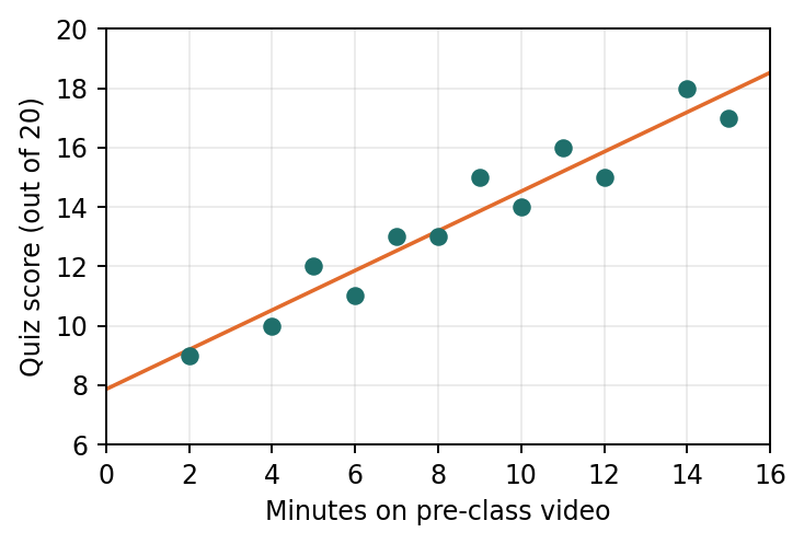
A teacher recorded, for 12 students, the number of minutes each student spent on a pre-class video (x) and the student's score on a 20-point quiz the next day (y). The scatterplot shows a strong, positive, linear association. Computer output for the least-squares regression is shown.

Scatterplot of quiz score against minutes on the video, with the regression line: a strong, positive, linear pattern
PredictorCoefSE CoefTP
Constant7.86250.562213.990.000
Minutes0.66650.059811.150.000

S = 0.7952     R-Sq = 92.6%

  1. (a) Write the equation of the least-squares regression line. Define any variables you use.
  2. (b) Interpret the slope of the regression line in context.
  3. (c) Interpret the value of R-Sq = 92.6% in context.
  4. (d) One student watched the video for 10 minutes and scored 14 on the quiz. Calculate and interpret this student's residual.
Show the model solution and scoring

Part (a)

Predicted quiz score = 7.8625 + 0.6665 (minutes of video watched).

  • Use the Constant row for the intercept and the Minutes row for the slope.
  • Here, score is the predicted quiz score (out of 20) and minutes is the number of minutes spent on the pre-class video.

Scoring. Essentially correct: correct equation, with a hat (or the word predicted) on the response and both variables defined in context.

Part (b)

For each additional minute spent on the video, the predicted quiz score increases by about 0.67 points.

  • For each additional minute a student spends on the pre-class video, the predicted quiz score increases by about 0.67 points.

Scoring. Essentially correct: says predicted (or average) score, gives 0.67 points per minute, and is in context. Partially correct: missing the word predicted, or stated as a certainty.

Part (c)

About 92.6% of the variation in quiz scores is accounted for by the linear relationship with minutes spent on the video.

  • About 92.6% of the variation in students' quiz scores is accounted for by the linear relationship between quiz score and minutes spent on the pre-class video.

Scoring. Essentially correct: refers to variation in quiz scores explained by the linear model with minutes. Partially correct: omits variation, the linear model, or context.

Part (d)

Predicted score ≈ 14.53, so the residual is 14 − 14.53 ≈ −0.53 points.

  • Residual = actual score − predicted score.
  • This student scored about 0.53 points lower than the regression line predicts for a student who watched 10 minutes.

Scoring. Essentially correct: correct prediction, residual of about −0.53, and an interpretation that says the actual score was below the predicted score, in context.

Unit 3

Designing a Flipped-Classroom Experiment

Collecting Data

A high school math department wants to know whether assigning short pre-class videos (a flipped approach) leads to higher unit test scores than a traditional in-class lecture. Eighty Grade 10 students at the school have volunteered to take part for one unit. Every student will take the same unit test at the end.

  1. (a) Describe how to randomly assign the 80 students to the two treatments so that each treatment has 40 students.
  2. (b) The department suspects that students' prior math grades (A or B, compared with C or below) are related to unit test scores. Describe how to use blocking in this experiment and explain why blocking is helpful here.
  3. (c) Suppose the video group's mean unit test score is significantly higher than the lecture group's. Can the department conclude that the video approach caused the higher scores? Can the results be generalized to all Grade 10 students in the country? Explain both answers.
  4. (d) A teacher suggests letting each student choose which approach to use instead of assigning them. Explain how this could lead to confounding.
Show the model solution and scoring

Part (a)

Number the students 1–80, use a random number generator to pick 40 different numbers, give those students the video approach and the other 40 the lecture.

  • Number the students from 1 to 80.
  • Use a random number generator to select 40 different integers from 1 to 80, ignoring repeats.
  • Students whose numbers are selected get the pre-class video approach; the remaining 40 students get the in-class lecture. (Writing the names on 80 identical slips, mixing them in a bag and drawing 40 also works.)

Scoring. Essentially correct: a random method that produces two groups of exactly 40, described clearly enough that two people could carry it out the same way.

Part (b)

Block by prior grade (A/B and C or below), randomly assign half of each block to each method, and compare within blocks.

  • Separate the students into two blocks: those with a prior grade of A or B, and those with C or below.
  • Within each block, randomly assign half of the students to the video approach and half to the lecture, then compare the treatments within each block.
  • Because prior grade is related to test scores, blocking removes that source of variation from the comparison. This makes it easier to detect a difference in scores caused by the teaching method.

Scoring. Essentially correct: blocks by prior grade, randomizes within blocks, and explains that blocking accounts for variation in scores due to prior grade. Partially correct: correct design but a weak explanation.

Part (c)

Yes to cause and effect for these students (random assignment); no to all Grade 10 students in the country (volunteers from one school, not a random sample).

  • Cause and effect: yes, for students like these. The treatments were randomly assigned, so the groups should be similar in every other way, and a significant difference can be attributed to the teaching method.
  • Generalization: no. The 80 students were volunteers from one school, not a random sample of Grade 10 students in the country, so the results apply only to students like these volunteers.

Scoring. Essentially correct: both conclusions, each tied to its reason (random assignment for causation, random sampling for generalization). Partially correct: one of the two.

Part (d)

Students who choose videos may be more motivated; motivation affects test scores, so its effect can't be separated from the method's.

  • Students who choose the video approach may be more motivated or more organized than students who choose the lecture.
  • Motivation is related to unit test scores and to the choice of method, so if the video group scores higher, we could not tell whether the method or the students' motivation caused the difference.

Scoring. Essentially correct: names a variable, explains how it is linked both to the choice of method and to test scores, and says the effects cannot be separated.

Unit 4

Video Language and Probability

Probability, Random Variables, and Probability Distributions

A random sample of 200 students who use an online math channel was asked which language version of the videos they prefer. The results, by grade, are shown.

EnglishFilipinoBothTotal
Grade 9304822100
Grade 10423622100
Total728444200
  1. (a) Find the probability that a randomly selected student from this sample prefers the Filipino version, given that the student is in Grade 9.
  2. (b) Are the events "student is in Grade 9" and "student prefers the Filipino version" independent? Justify your answer.
  3. (c) Across the whole channel, 30% of viewers choose the Filipino version. Suppose 10 viewers are selected at random, and let X be the number who choose the Filipino version. Find P(X = 3) and P(X ≥ 1). Show your work.
  4. (d) Find the mean and standard deviation of X, and interpret the mean in context.
Show the model solution and scoring

Part (a)

P(Filipino | Grade 9) = 48 ÷ 100 = 0.48.

  • Restrict attention to the 100 Grade 9 students; 48 of them prefer the Filipino version.

Scoring. Essentially correct: 0.48 with the correct denominator shown.

Part (b)

No. P(Filipino) = 84 ÷ 200 = 0.42, which is not equal to P(Filipino | Grade 9) = 0.48.

  • The events are not independent. If they were, the probability of preferring Filipino would be the same whether or not we know the student is in Grade 9.
  • Overall, 42% of students prefer Filipino, but 48% of Grade 9 students do. Knowing the grade changes the probability.

Scoring. Essentially correct: compares the two correct probabilities (or an equivalent check) and concludes not independent.

Part (c)

X is binomial with n = 10, p = 0.30. P(X = 3) ≈ 0.2668 and P(X ≥ 1) = 1 − 0.710 ≈ 0.9718.

  • X has a binomial distribution with n = 10 and p = 0.30: there is a fixed number of trials, each viewer either chooses Filipino or not, and viewers are independent (10 is far less than 10% of all viewers).
  • For P(X ≥ 1), use the complement: the only way to get fewer than 1 is for none of the 10 to choose Filipino.

Scoring. Essentially correct: identifies the binomial distribution with n and p, and gets both probabilities with work or labeled calculator inputs (binompdf, binomcdf).

Part (d)

Mean = 3 viewers; standard deviation ≈ 1.449 viewers. Over many random samples of 10 viewers, the average number choosing Filipino would be about 3.

  • Interpretation: if we took many random samples of 10 viewers, the average number who choose the Filipino version would be about 3 per sample.

Scoring. Essentially correct: both values and an interpretation that refers to the long-run average over many samples, in context.

Unit 5

Smartphones With Mobile Data

Sampling Distributions

In a large school district, 62% of high school students have a smartphone with mobile data. A researcher plans to select a random sample of 150 high school students from the district and find the proportion of the sample who have a smartphone with mobile data.

  1. (a) Find the mean and standard deviation of the sampling distribution of the sample proportion. Show that any condition needed for your standard deviation formula is met.
  2. (b) Explain why the sampling distribution of the sample proportion is approximately normal.
  3. (c) Find the probability that 55% or fewer of the students in the sample have a smartphone with mobile data.
  4. (d) How would the standard deviation of the sampling distribution change if the sample size were 600 instead of 150? Explain.
Show the model solution and scoring

Part (a)

Mean = 0.62; standard deviation = √(0.62 × 0.38 ÷ 150) ≈ 0.0396.

  • The standard deviation formula requires the 10% condition: 150 students is less than 10% of all high school students in a large district.

Scoring. Essentially correct: both values and the 10% condition stated in context.

Part (b)

Large Counts: 150(0.62) = 93 and 150(0.38) = 57 are both at least 10.

  • The Large Counts condition is met: the expected numbers of successes and failures are both at least 10, so the sampling distribution is approximately normal.

Scoring. Essentially correct: both counts calculated and compared with 10.

Part (c)

z = (0.55 − 0.62) ÷ 0.0396 ≈ −1.77, so the probability is about 0.0387 (0.0384 from a table with z = −1.77).

  • Use the normal distribution with mean 0.62 and standard deviation 0.0396, and find the area to the left of 0.55.
  • There is only about a 4% chance that a random sample of 150 students would include 55% or fewer with mobile data.

Scoring. Essentially correct: correct normal distribution and boundary shown, with an answer of about 0.038 or 0.039.

Part (d)

It would be cut in half, to about 0.0198, because the sample size is 4 times as large and the SD depends on 1 ÷ √n.

  • The sample size is multiplied by 4, and the standard deviation is divided by the square root of n, so it is divided by 2.
  • Larger random samples give sample proportions that vary less from sample to sample.

Scoring. Essentially correct: says the standard deviation is halved (about 0.0198) and explains why.

Unit 6

Studying Math With Online Videos

Inference for Categorical Data: Proportions

A national survey reports that 40% of high school students use online videos to study math at least once a week. A teacher believes the proportion is higher at her school, which has about 3,000 students. She selects a random sample of 200 students from her school, and 96 of them say they use online videos to study math at least once a week.

  1. (a) State the null and alternative hypotheses for a test of the teacher's belief. Define the parameter.
  2. (b) Check the conditions for a one-sample z test for a proportion, then calculate the test statistic and the P-value.
  3. (c) What conclusion should the teacher make at the α = 0.05 significance level? Explain in context.
  4. (d) Describe a Type I error in the context of this study.
Show the model solution and scoring

Part (a)

H0: p = 0.40 versus Ha: p > 0.40, where p is the proportion of all students at her school who use online videos to study math at least once a week.

  • p is the proportion of all students at the teacher's school who use online videos to study math at least once a week.

Scoring. Essentially correct: correct hypotheses using a parameter, and the parameter defined in context.

Part (b)

Random sample; 200 < 10% of 3,000; 200(0.40) = 80 and 200(0.60) = 120 are at least 10. Sample proportion = 0.48, z ≈ 2.31, P-value ≈ 0.0105.

  • Random: the 200 students are a random sample from the school.
  • 10%: 200 is less than 10% of the school's 3,000 students.
  • Large Counts: 200(0.40) = 80 and 200(0.60) = 120 are both at least 10.

Scoring. Essentially correct: all three conditions checked, and a correct test statistic and P-value with the formula or labeled calculator inputs (1-PropZTest).

Part (c)

Because 0.0105 < 0.05, reject H0. There is convincing evidence that more than 40% of students at her school use online videos to study math weekly.

  • Because the P-value of 0.0105 is less than α = 0.05, we reject H0.
  • There is convincing evidence that the proportion of all students at the teacher's school who use online videos to study math at least once a week is greater than 0.40.

Scoring. Essentially correct: compares the P-value with α, makes the correct decision, and states the conclusion about the population proportion in context, without saying the null is proven false.

Part (d)

Concluding that more than 40% of students at her school use videos weekly when the true proportion is actually 40%.

  • A Type I error would be concluding that more than 40% of students at the school use online videos to study math weekly, when in fact the true proportion is 40%.

Scoring. Essentially correct: rejecting a true null, described in context.

Unit 7

Quiz Scores Before and After Review Videos

Inference for Quantitative Data: Means

A teacher added short review videos to a unit. Ten students, selected at random from the teacher's 120 students, took a 50-point quiz on the unit before watching the videos and a similar quiz after watching them. Their scores are shown.

Student12345678910
Before31283540253337294230
After35303841313440334336
  1. (a) Explain why a paired t procedure is appropriate here, rather than a two-sample t procedure.
  2. (b) Do the data provide convincing evidence, at the α = 0.05 level, that students' mean score increases after watching the review videos? Give appropriate statistical evidence.
  3. (c) Construct and interpret a 95% confidence interval for the mean difference in scores (after − before).
  4. (d) Can the teacher conclude that watching the review videos caused the increase in scores? Explain.
Show the model solution and scoring

Part (a)

Each student was measured twice, so the before and after scores are dependent pairs; analyze the differences.

  • The same 10 students took both quizzes, so each before score is paired with an after score from the same student.
  • The two sets of scores are not independent samples, so we analyze the differences (after − before).

Scoring. Essentially correct: says the same students were measured twice, so the data are paired or dependent.

Part (b)

Differences (after − before): 4, 2, 3, 1, 6, 1, 3, 4, 1, 6. Mean difference = 3.1, SD ≈ 1.912, t ≈ 5.13 with df = 9, P-value ≈ 0.0003. Reject H0.

  • The differences (after − before) are 4, 2, 3, 1, 6, 1, 3, 4, 1, 6.
  • H0: the mean difference is 0. Ha: the mean difference is greater than 0, where the mean difference is the true mean of (after − before) for all 120 of the teacher's students.
  • Conditions: the 10 students were selected at random; 10 is less than 10% of the teacher's 120 students; and a dotplot of the differences shows no strong skew or outliers, so a t procedure is reasonable with n = 10.
  • Because the P-value of about 0.0003 is less than 0.05, reject H0. There is convincing evidence that the mean quiz score for the teacher's students increases after watching the review videos.

Scoring. Essentially correct: hypotheses with a defined parameter, conditions (including a check of the differences for normality), correct mechanics, and a conclusion in context linked to the P-value.

Part (c)

3.1 ± 2.262(1.912 ÷ √10) gives (1.73, 4.47) points.

  • Use t* = 2.262 for 95% confidence with df = 9.
  • We are 95% confident that the interval from 1.73 to 4.47 points captures the true mean increase in quiz score (after − before) for the teacher's students.

Scoring. Essentially correct: correct interval with work and an interpretation about the true mean difference, in context.

Part (d)

No. There was no control group or random assignment; the increase could come from taking a second quiz or extra study time.

  • No. This was not an experiment with a control group: every student watched the videos, and there was no random assignment of treatments.
  • The increase could be due to other things, such as practice from taking the first quiz or extra studying between quizzes.

Scoring. Essentially correct: says no, with a reason based on the lack of a control group or random assignment, and names a plausible alternative explanation.

Unit 8

Favorite Study Resource by Grade

Inference for Categorical Data: Chi-Square

A large high school selected separate random samples of 100 students from each of Grades 9, 10 and 11. Each grade has more than 1,000 students. Each student was asked which resource helps them most when studying for a math test. The results are shown.

VideosTextbookTutor or classmateTotal
Grade 9523018100
Grade 10453322100
Grade 11333730100
Total13010070300
  1. (a) Identify the appropriate chi-square test and state the hypotheses.
  2. (b) Calculate the expected count of Grade 9 students who prefer videos, and show that the conditions for the test are met.
  3. (c) The test statistic is χ² = 8.20. Find the degrees of freedom and the P-value, and state a conclusion at the α = 0.05 level.
  4. (d) Which cell contributes most to the chi-square statistic? What does that cell suggest?
Show the model solution and scoring

Part (a)

Chi-square test for homogeneity. H0: the distribution of preferred study resource is the same for all three grades. Ha: the distributions are not all the same.

  • The school took separate random samples from three grades and recorded one categorical variable, so this is a chi-square test for homogeneity.
  • H0: the distribution of preferred study resource is the same for Grade 9, Grade 10 and Grade 11 students at the school. Ha: the distribution is not the same for all three grades.

Scoring. Essentially correct: names the homogeneity test (with a reason) and states hypotheses about the distributions in context.

Part (b)

Expected = 100 × 130 ÷ 300 ≈ 43.33. All expected counts are at least 23.33, so all are at least 5.

  • Random: separate random samples were taken from each grade.
  • 10%: 100 students is less than 10% of each grade (each has more than 1,000).
  • Large Counts: the smallest expected count is 100(70) ÷ 300 ≈ 23.33, so all expected counts are at least 5.

Scoring. Essentially correct: correct expected count with work and all three conditions checked.

Part (c)

df = 4 and the P-value ≈ 0.085. Because 0.085 > 0.05, fail to reject H0: there is not convincing evidence that the distributions differ by grade.

  • Because the P-value of about 0.085 is greater than α = 0.05, we fail to reject H0.
  • There is not convincing evidence that the distribution of preferred study resource differs among Grade 9, 10 and 11 students at this school. (This does not prove the distributions are the same.)

Scoring. Essentially correct: correct df and P-value, the correct decision, and a conclusion in context that does not accept H0.

Part (d)

Grade 11 / Videos contributes about 2.46: fewer Grade 11 students chose videos (33) than expected (43.33) if the distributions were the same.

  • The Grade 11, Videos cell contributes the most, about 2.46 of the 8.20.
  • Fewer Grade 11 students named videos (33) than we would expect (43.33) if all three grades had the same distribution. Even so, the overall test did not find convincing evidence of a difference.

Scoring. Essentially correct: identifies the cell with its contribution and compares observed with expected in context.

Unit 9

Practice Hours and Test Scores

Inference for Quantitative Data: Slopes

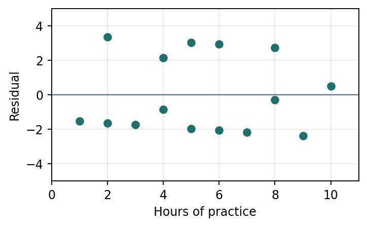
A random sample of 15 students was selected from a large high school. For each student, a teacher recorded the number of hours spent on practice worksheets in the week before a unit test (x) and the student's test score as a percent (y). Computer output from a least-squares regression and a residual plot are shown.

PredictorCoefSE CoefTP
Constant60.43231.345544.910.000
Hours3.10650.226413.720.000

S = 2.301     R-Sq = 93.5%

Residual plot: residuals scattered randomly above and below zero with no curve and similar spread
  1. (a) Construct a 95% confidence interval for the slope of the population regression line relating test score to hours of practice.
  2. (b) Interpret the interval in context.
  3. (c) Does the interval provide convincing evidence of a positive linear relationship between hours of practice and test score for all students at the school? Explain.
  4. (d) Explain what the residual plot tells you about the conditions for inference about the slope.
Show the model solution and scoring

Part (a)

3.1065 ± 2.160(0.2264) gives (2.62, 3.60), using t* = 2.160 with df = 13.

  • The slope is 3.1065 and its standard error is 0.2264 (the Hours row).
  • With n = 15, df = 15 − 2 = 13, so t* = 2.160 for 95% confidence.
  • 3.1065 ± 0.489 gives about 2.62 to 3.60.

Scoring. Essentially correct: correct values from the output, correct df and t*, and the correct interval.

Part (b)

We are 95% confident that the interval from 2.62 to 3.60 captures the slope of the true regression line: for each additional hour of practice, the average test score increases by between 2.62 and 3.60 percentage points.

  • We are 95% confident that the interval from 2.62 to 3.60 captures the slope of the population regression line.
  • That is, for each additional hour of practice, the average test score for students at this school increases by between about 2.62 and 3.60 percentage points.

Scoring. Essentially correct: refers to the population slope (true average change) and gives both endpoints in context.

Part (c)

Yes. Every value in the interval is greater than 0, so a slope of 0 (no linear relationship) is not plausible.

  • Yes. All values in the interval are positive, so 0 is not a plausible value for the population slope.

Scoring. Essentially correct: says yes because 0 (or any negative value) is not in the interval.

Part (d)

No curved pattern (linear condition met) and roughly constant spread (equal standard deviation condition met).

  • The residuals are scattered randomly above and below 0 with no curved pattern, so a linear model is appropriate.
  • The spread of the residuals is about the same across all values of x, so the condition of equal standard deviation of y for each x is reasonable.

Scoring. Essentially correct: addresses both linearity (no curve) and equal variability (no fanning), referring to the plot.

Video walkthroughs of released exam questions

Dr. E solves free-response questions from released AP Statistics exams, step by step. Get the official questions from AP Central, try them, then watch.

FRQ

AP Exam Free-Response Walkthroughs

6 released-exam walkthroughs · the Filipino toggle shows a related concept lesson
▾

← Back to the AP Statistics lessons by unit · Teaching AP Stats? Read the flipping guide